ClioSport.net

Register a free account today to become a member!
Once signed in, you'll be able to participate on this site by adding your own topics and posts, as well as connect with other members through your own private inbox!

  • When you purchase through links on our site, we may earn an affiliate commission. Read more here.

Spreadsheet Assistance


Yo!
I'm in the process of trying to sort a simple sheet (in theory) to track some information at work. However, I'm struggling.

The idea is to have engineers listed in the drop box below ENGINEER below.
This is where it gets a bit tricky.
What I want is for the day rate for the selected engineer then appear in the DAY RATE column - this column will be hidden eventually. But I'll use the info in this column to complete the rest of the sheet.
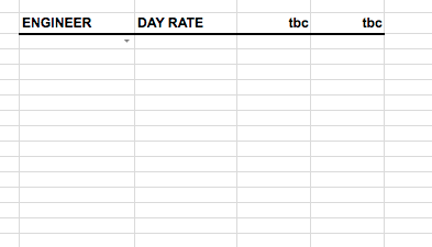
Screen Shot 2017-12-14 at 10.47.38.png


I feel like I did this type of thing years ago at school but can't for the life of me remember how to do it! Google has proved a bit fruitless so far.

This is Google Sheets by the way.

Any assistance appreciated.
 

boultonn

ClioSport Club Member
  Macan S
Hello jam.
Put the engineers and their corresponding day rate in a second sheet, then the function you're looking for is vlookup
Hope this helps
 
  Clio Sport 182
Create a table of the engineers and their daily rates. Then do a validation in the engineer cells using the engineers column from the table above (that'll give you a drop down of the engineers names to select from). Then in the daily rate column do a vlookup of the selected engineers name from the table of engineers and rates. Hope that helps - if you're not familiar with validation or vlookup then you may need a hand.

Sent from my SM-G955F using Tapatalk
 
Thanks chaps - I'd already set up another sheet with engineers names on (Which would feed the drop down menu). Then following this () tutorial I've created the below (engineers and day rates are not true believe it or not)
Screen Shot 2017-12-14 at 12.50.25.png


however, when I go to the sheet I want it to output - I get this..
Screen Shot 2017-12-14 at 12.56.01.png


this is the formula I'm using - the range was named to INFO..
Screen Shot 2017-12-14 at 12.56.11.png


hmm...

duncecap.jpg
 

Oggy997

ClioSport Club Member
  997.1, Caddy, e208
I use index/match as it's more versatile than Vlookup.

It's
=index(dayratecolumn,match(engineer,engineercolumn,0))
 

sburrell93

Scotland - South
ClioSport Area Rep
I think you need to reference the other sheet. Instead of just using B11 as the reference try 'sheet2!B11' (replace sheet2 with whatever the sheet is actually called).

Not really used vlookup before mind you so may be wrong.
 

Chrisgti6

ClioSport Club Member
  Too many
The issue in your vlookup is you've told it to give you the values from column 3, but your table only contains 2 columns. Change the 3 to a 2.
 
I use index/match as it's more versatile than Vlookup.

It's
=index(dayratecolumn,match(engineer,engineercolumn,0))
interesting - how does that break down? I assume dayratecolumn and engineercolumn are just references to the said column in the other sheet? what does engineer then represent?

I did what I thought may be correct, but got the below..
Screen Shot 2017-12-14 at 15.29.35.png
 
I think you need to reference the other sheet. Instead of just using B11 as the reference try 'sheet2!B11' (replace sheet2 with whatever the sheet is actually called).

Not really used vlookup before mind you so may be wrong.

I'm confused why I'd need to reference the other sheet here - the B11 merely relates to the engineer that has been selected from the drop down menu (of which is stored on the other sheet).
 

Oggy997

ClioSport Club Member
  997.1, Caddy, e208
I wouldnt use whole columns, but may explain easier.
 

Attachments

  • cs.png
    cs.png
    36.9 KB · Views: 60

Oggy997

ClioSport Club Member
  997.1, Caddy, e208
If you have skype or some form of desktop based messaging client Im happy to help you over that?
 

Ay Ay Ron

ClioSport Club Member
Bumping this.

@MarkCup might be able to do this in a nanosecond.


I've got a list which is set at 5 minute intervals for the year of 2023.

I need to select in column C a range between 4.60 & 4.80. Then I need to put it into another sheet so I can select a few times for each day (for access to a tidal port)

IMG_20230420_165945.jpg


If I search for 4.7 I can find them all but the dates don't show (as above, it just shows book, sheet, etc, but no date)
Couldn't see a range to search for though.
 

Oggy997

ClioSport Club Member
  997.1, Caddy, e208
I need to select in column C a range between 4.60 & 4.80. Then I need to put it into another sheet so I can select a few times for each day (for access to a tidal port)
Can you elaborate on that further, I have no idea what you are actually aiming to do
 

Ay Ay Ron

ClioSport Club Member
Can you elaborate on that further, I have no idea what you are actually aiming to do
I'll try.
The document I have is 400+ pages long. I want to sorted the data to heights I'm only concerned about.

Column A is the date.
Column B is the time (5 minute intervals).
Column C is the tide height.

I want the range for the tide height between 4.6 & 4.8 for every day of the year.

I then can put down when it's a safe entry into the port so we don't go aground. I have to do sail times including access restrictions for each month. From May it's been made harder by the inclusion of another boat and a spastic crew who can't do anything for themselves. (I don't have to do this for my boat as we use a different method)

Ie. When it's 4.7m I know the boat can safely get in but if I just search for 4.7 it searches for 4.70 and the data only has that for certain days hence me needing a range which should show something for every day.

Hopefully that's explained it a bit better 😂
 

TheEvilGiraffe

South East - Essex
ClioSport Area Rep
I'll try.
The document I have is 400+ pages long. I want to sorted the data to heights I'm only concerned about.

Column A is the date.
Column B is the time (5 minute intervals).
Column C is the tide height.

I want the range for the tide height between 4.6 & 4.8 for every day of the year.

I then can put down when it's a safe entry into the port so we don't go aground. I have to do sail times including access restrictions for each month. From May it's been made harder by the inclusion of another boat and a spastic crew who can't do anything for themselves. (I don't have to do this for my boat as we use a different method)

Ie. When it's 4.7m I know the boat can safely get in but if I just search for 4.7 it searches for 4.70 and the data only has that for certain days hence me needing a range which should show something for every day.

Hopefully that's explained it a bit better 😂

Select your data

Filter

Conditional formatting on the colour you want .. if x to y .. colour it.

Then filter by colour.

Then copy visibile leftovers into a new tab to get just that.

Or something.
 
I'll try.
The document I have is 400+ pages long. I want to sorted the data to heights I'm only concerned about.

Column A is the date.
Column B is the time (5 minute intervals).
Column C is the tide height.

I want the range for the tide height between 4.6 & 4.8 for every day of the year.

I then can put down when it's a safe entry into the port so we don't go aground. I have to do sail times including access restrictions for each month. From May it's been made harder by the inclusion of another boat and a spastic crew who can't do anything for themselves. (I don't have to do this for my boat as we use a different method)

Ie. When it's 4.7m I know the boat can safely get in but if I just search for 4.7 it searches for 4.70 and the data only has that for certain days hence me needing a range which should show something for every day.

Hopefully that's explained it a bit better 😂
Would just adding a filter to the tab hel. Then select only 4.6 - 4.8 tide height to display.


Not that anyone cares, but I gave up on the original query from all those years ago. I found a workaround, I was just making it harder than it was.

I'm now in a role where I've made an absolute dream of a spreadsheet that contains everything I need on a daily basis. vlookups, filters and colours all over the shop. It's made my job so much easier.
 

Oggy997

ClioSport Club Member
  997.1, Caddy, e208
Would just adding a filter to the tab hel. Then select only 4.6 - 4.8 tide height to display.


Not that anyone cares, but I gave up on the original query from all those years ago. I found a workaround, I was just making it harder than it was.

I'm now in a role where I've made an absolute dream of a spreadsheet that contains everything I need on a daily basis. vlookups, filters and colours all over the shop. It's made my job so much easier.

You mean I waited 6 years to find out you didnt care for my thorough explanation?

Select your data

Filter

Conditional formatting on the colour you want .. if x to y .. colour it.

Then filter by colour.

Then copy visibile leftovers into a new tab to get just that.

Or something.

No need for colours, just filter the number betwen 4.6 - 4.8

1682012631959.png


1682012657169.png


If you wanted a macro to filter

Code:
Sub AyAyRon()

With ActiveSheet
        lastr0w = .Cells(.Rows.Count, "C").End(xlUp).Row
    End With

    ActiveSheet.Range("$C$1:$C$" & lastr0w).AutoFilter Field:=1, Criteria1:=">=4.6", _
        Operator:=xlAnd, Criteria2:="<=4.8"
End Sub

and to copy to a new sheet called GayGayRon

Code:
Sub AyAyRon()

With ActiveSheet
        lastr0w = .Cells(.Rows.Count, "C").End(xlUp).Row
    End With

    ActiveSheet.Range("$C$1:$C$" & lastr0w).AutoFilter Field:=1, Criteria1:=">=4.6", _
        Operator:=xlAnd, Criteria2:="<=4.8"
        
        
ActiveSheet.Range("$A$1:$C$" & lastr0w).SpecialCells(xlCellTypeVisible).Copy Destination:=Sheets("GayGayRon").Range("A1")
End Sub
 

Ay Ay Ron

ClioSport Club Member
Cheers guys.
Done the filter thing and have now copied May's over to another page. Just needed pictures to assist.
Will do the same for each other month tomorrow.

I was halfway through the colour thing but I pressed something and it went south.

I genuinely think my 2 year old would have a better understanding of this than me.

What the f**k is a macro 😂
 

Oggy997

ClioSport Club Member
  997.1, Caddy, e208
All the steps automated, using visual basic.
So if you do this daily, it can become 1 click.
 
Hi chaps,

I have one spreadsheet that I need to ideally VLOOKUP some data from another sheet (full of mass project data).

I have used VLOOKUPs all over the place on this, however, this is a bit tricky as the data I'm referring to could be anything from one line to 30+ lines of data so I'm not sure how to go about it...

I've found FILTER may be where I want to get to but not getting where I need to at the minute...

The below is a quick idea of what I need;

This is where all the (fascinating in this case) data is stored


7EA60484-DC98-403D-BA26-319626A564B6.png


And this is where I will need it to display, dependent upon the project number akin to a vlookup.
AB4C95D2-FBC6-4634-B82E-EF79106B0E37.png
 

Oggy997

ClioSport Club Member
  997.1, Caddy, e208
Ok, cell E7

=IF(INDEX(Sheet1!D: D,MATCH(Sheet2!$D$3,Sheet1!$C:$C,0))=0,"",INDEX(Sheet1!D: D,MATCH(Sheet2!$D$3,Sheet1!$C:$C,0)))

This can be dragged left to right - this will find match#1

For nth matching we need to use an array formula (and you cant drag it down sadly) - to perform an array formula, you must confirm the formula with CSE (Ctrl+s**t+Enter) - your formula will be enclosed in {}

The red number is the result number

e.g. E8

=IF(INDEX(Sheet1!D: D,SMALL(IF(Sheet2!$D$3=Sheet1!C:C,ROW(Sheet1!C:C)-ROW(Sheet1!$C$1)+1),2))=0,"",INDEX(Sheet1!D: D,SMALL(IF(Sheet2!$D$3=Sheet1!C:C,ROW(Sheet1!C:C)-ROW(Sheet1!$C$1)+1),2)))

E9

=IF(INDEX(Sheet1!D: D,SMALL(IF(Sheet2!$D$3=Sheet1!C:C,ROW(Sheet1!C:C)-ROW(Sheet1!$C$1)+1),3)=0,"",INDEX(Sheet1!D: D,SMALL(IF(Sheet2!$D$3=Sheet1!C:C,ROW(Sheet1!C:C)-ROW(Sheet1!$C$1)+1),3)))

I can write code to fill this formula down for you rather than you type it manually each time, but I would need the exact sheetnames and ranges etc (if it's not sensitive data, you can send me the sheet to cliosport@ogilv.ie )
 
Ok, cell E7


This can be dragged left to right - this will find match#1

For nth matching we need to use an array formula (and you cant drag it down sadly) - to perform an array formula, you must confirm the formula with CSE (Ctrl+s**t+Enter) - your formula will be enclosed in {}

The red number is the result number

e.g. E8


E9


I can write code to fill this formula down for you rather than you type it manually each time, but I would need the exact sheetnames and ranges etc (if it's not sensitive data, you can send me the sheet to cliosport@ogilv.ie )
Really appreciate you taking the time to do that.

One thing though, sheet 2 (where I would like all the data to appear) is essentially a summary sheet as no static data is stored there. Whenever I enter the project number in the yellow box, loads of information relating to that project is pulled from numerous sheets to give a quick overview of loads of data specific to that project. With this in mind, how would the formula above reference the store number as it would change on an adhoc basis? Apolgies if I missed it!
 

Oggy997

ClioSport Club Member
  997.1, Caddy, e208
Im not sure i understand your queation, i used cell Sheet2!$D$3 as a lookup value
 

Oggy997

ClioSport Club Member
  997.1, Caddy, e208
@jam. everything ok? Ive kept a copy of your workbook template that I'd like to tidy up if so.
 
@jam. everything ok? Ive kept a copy of your workbook template that I'd like to tidy up if so.
It was going great, I was amending the formulas etc to suit my sheets then boom the sheet I am referencing has been updated to a different layout so I need to do some rearranging to make it work again.


Top